Branching Recursion
A recursive function may have multiple base cases or make several recursive calls. The number and expense of those calls can drastically increase or reduce computation time.
Example: Fibonacci Numbers
The Fibonacci numbers \(F_0, F_1, F_2, \ldots\) are defined recursively by
Each number after the first two is the sum of the previous two: \(0, 1, 1, 2, 3, 5, 8, 13, \ldots\). This definition has two base cases, \(F_0 = 0\) and \(F_1 = 1\), and a recursive case that refers to two smaller Fibonacci numbers. A recursive implementation calls itself twice in the recursive case.
def fib(n):
    """Compute the Fibonacci number F_n recursively."""
    if n == 0:  # Base case: F_0 = 0.
        return 0
    if n == 1:  # Base case: F_1 = 1.
        return 1
    return fib(n - 1) + fib(n - 2)  # Recursive case: two calls.


print([fib(n) for n in range(10)])
[0, 1, 1, 2, 3, 5, 8, 13, 21, 34]
Each call with \(n \geq 2\) makes two more calls, so the total number of calls can be visualized as a tree.
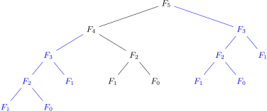
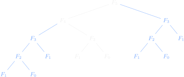
The work shown in blue is done twice: fib(5) and fib(4) both call fib(3), which computes the same value from scratch each time.
Similarly, fib(2) is computed three times.
The code closely follows the mathematical definition, but the repeated work compounds quickly.
In total, fib(n) makes \(2F_{n+1} - 1\) calls, a number that grows exponentially with \(n\).
\(n\) |
Number of function calls made by |
|---|---|
10 |
177 |
20 |
21,891 |
30 |
2,692,537 |
40 |
331,160,281 |
An iterative approach is much more efficient than this direct recursive implementation.
Faster Recursion
Recursion alone does not necessarily make an algorithm faster. The speedup usually comes from one or more of the following.
Halving the problem size. Recursing on \(n/2\) instead of \(n - 1\) reaches a base case in about \(\log_2(n)\) steps instead of \(n\) steps.
Reducing the number of recursive branches. One recursive call per step instead of two avoids building a tree of calls.
Caching the solutions of repeated subproblems. Storing the value of
fib(3)the first time it is computed avoids computing it again. This is called memoization (not memorization!).
The following examples use the first strategy, halving the problem size.
Problem 3
The Fibonacci numbers satisfy the doubling identities
Write a function named fib_pair() that accepts a nonnegative integer \(n\) and computes \(F_n\) and \(F_{n+1}\) as follows.
If \(n = 0\), this is the base case: return \(F_0 = 0\) and \(F_1 = 1\).
Otherwise, let \(k = \lfloor n/2 \rfloor\) and call
fib_pair()once to get \(F_k\) and \(F_{k+1}\).
Here, \(k = \lfloor n/2 \rfloor\) (integer division) when \(n = 2k\) or \(n = 2k + 1\).Use the formulas above to compute \(F_{2k}\) and \(F_{2k+1}\).
If \(n\) is even, then \(F_n = F_{2k}\) and \(F_{n+1} = F_{2k+1}\).
If \(n\) is odd, then \(F_n = F_{2k+1}\) and \(F_{n+1} = F_{2k} + F_{2k+1}\).
Return \(F_n\) and \(F_{n+1}\).
Test Cases
When implemented correctly, fib_pair(200) makes 9 calls, while fib(200) would require about \(9 \times 10^{41}\) calls.
print(fib_pair(0))
print(fib_pair(1))
print(fib_pair(10))
print(fib_pair(200))
(0, 1)
(1, 1)
(55, 89)
(280571172992510140037611932413038677189525, 453973694165307953197296969697410619233826)
Problem 4
The matrix power \(A^n = AA\cdots A\) (\(n\) times) of a square matrix \(A\) satisfies
where \(I\) is the identity matrix.
Write a function named matrix_power() that accepts a square NumPy array \(A\) and a nonnegative integer \(n\).
Compute \(A^n\) recursively using the formulas above.
Reminder: np.eye(m) creates the \(m \times m\) identity matrix.
Test Cases
import numpy as np

B = np.array([
    [1, 1],
    [1, 0],
])
print(matrix_power(B, 0))
print(matrix_power(B, 1))
print(matrix_power(B, 10))
print(matrix_power(B, 200))
[[1. 0.]
 [0. 1.]]
[[1. 1.]
 [1. 0.]]
[[89. 55.]
 [55. 34.]]
[[4.53973694e+41 2.80571173e+41]
 [2.80571173e+41 1.73402521e+41]]
Fun fact: the powers of \(B = \left[\begin{array}{cc} 1 & 1 \\ 1 & 0 \end{array}\right]\) contain Fibonacci numbers! For \(n \ge 1\),